Someone emailed me recently and asked about how APT uses random matrix theory in their factor model. Another question I was asked is whether my package tawny could be used to replace APT or any other multi-factor model. The short answer is no. The slightly longer answer is that if you want to estimate a covariance matrix to use for portfolio optimization, you can use tawny for that purpose. In the next version, other methods of constructing the correlation matrix will be provided. Note that depending on the purpose of the covariance matrix (risk estimates versus portfolio optimization), different techniques for constructing the covariance matrix are appropriate. I’ll discuss this in more detail in a later post.

Back to this post… Typically RMT is used in covariance matrix estimation as a null hypothesis to remove eigenvalues associated with noise. APT’s global daily model is a statistical factor model [1], and the methodology they describe is to choose the number of factors for their multi-factor model based on the upper cutoff of the noise spectrum.

It is easy to deconstruct the model and validate its parameters as they are using a standard Marcenko Pastur distribution to fit the eigenvalues.

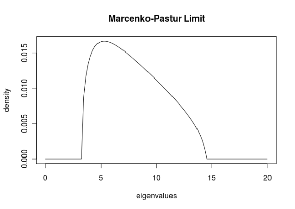
Since the paper provides the Q value and the lower and upper eigenvalue bounds, we can recreate the Marcenko Pastur limit for these parameters. First, let’s verify that the model is as we suppose [A] using futile.matrix:

> model <- create(WishartModel,8181,1044, sd=1) > domain(model) [1] 3.237562 14.434852

So the upper and lower bounds match the documentation. Below is the full spectrum for this Q (and variance):

Unfortunately the document does not provide all the calculated eigenvalues, but they do provide the top 100. We can use a subset of these and overlay the theoretical distribution on a histogram of the eigenvalues of the return series to get a sense of the fit [B]. It appears that this fit is reasonable, but without the remaining data we cannot be conclusive.

Through this exercise, we delved into the APT methodology and illustrated how random matrix theory can be applied to finance. In a later post, we’ll look at constructing our own statistical factor model and see what performance it provides.

Code Listings

[A]  Upper and lower eigenvalue bounds

> library(futile.matrix)
> model <- create(WishartModel,8181,1044)
> domain(model)
[1] 3.237562 14.434852

[B] Theoretical limit of eigenvalue spectrum

> xs <- seq(10,20, length.out=40)
> hist(es[es<20], breaks=20, xlab='eigenvalues', main='Eigenvalues of the APT daily global model')
> lines(xs, dmp(xs, svr=Q)*950)

References

[1] http://www.sungard.com/~/media/Campaigns/FinancialSystems/AlternativeInvestments/APT_Daily_Risk_Models_Whitepaper.ashx